Importance Sample BRDF

1 Summary

本文主要介绍微表面模型的 BRDF 的重要性采样过程，即使用重要性采样来计算渲染方程的积分。

2 Background

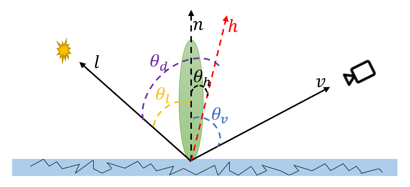
假设如下图所示的反射过程：

Fig 1: 微表面反射图示

有渲染方程
$$
L_o(P, \boldsymbol{v})=L_e(P, \boldsymbol{v})+\int_{\Omega^+}L_i(\boldsymbol{l})f(\boldsymbol{l}, \boldsymbol{v}) \cos\theta_l \space d\boldsymbol{l}
$$

其中 $P$ 为着色点，$\boldsymbol{l}$ 为入射光方向(指向光源)，$\boldsymbol{v}$ 为观察方向；第一项 $L_e$ 为着色点 $P$ 自发光，第二项为反射光，记为 $L_r$，本文主要关注第二项。第二项中 $L_i(\boldsymbol{l})$ 为入射光的属性，如颜色等；$f(\boldsymbol{l},\boldsymbol{v})$ 为 BRDF，本文只关注 microfacet BRDF。注意这里的 $\boldsymbol{l}$ 相当于单位立体角的方向，其他地方常记作 $\omega_i$ ，反射项的积分即在法线方向的半球上对立体角的积分。

2.1 蒙特卡洛积分

$L_r$ 积分没有解析解，直接求复杂很高，通常使用蒙特卡洛求积分的估计值。假设要求积分 $\int f(x) \space dx$，并且自变量服从一个分布 $X \sim P(x)$，概率密度为 $p(x)$。这时我们可以在积分区间内，以分布 $X \sim p(x)$ 进行很多次采样，得到 $X_1, X_2, …, X_N$。使用这些采样点可以得到积分的估计，方法如下：
$$
\int f(x) \space dx = \int \frac{f(x)}{p(x)}\cdot p(x) \space dx=E\left[\frac{f(x)}{p(x)}\right]
$$
我们将求积分转为了求期望 $E\left[\frac{f(x)}{p(x)}\right]$，对于期望，可以进行无偏估计(样本均值)：
$$
E\left[\frac{f(x)}{p(x)}\right] \approx \frac{1}{N}\sum\limits_{i=1}^{N}\frac{f(X_i)}{p(X_i)}
$$
将采样点代入上式，即可得到积分的估计。

使用蒙特卡洛积分后的 $L_r$
$$
L_r=\int_{\Omega^+}L_i(\boldsymbol{l})f(\boldsymbol{l}, \boldsymbol{v}) \cos\theta_l \space d\boldsymbol{l}\approx\frac{1}{N}\sum\limits_{k=1}^N\frac{L_i(\boldsymbol{l}_k)f(\boldsymbol{l}k,\boldsymbol{v})\cos\theta{l_k}}{p(\boldsymbol{l}_k)} \tag{1} \label{BRDF MC}
$$
想要求上述积分，除了很多采样点之外，还需要知道 $\boldsymbol{l}$ 的概率密度 $p(\boldsymbol{l})$，而这个概率密度的选取要尽量接近被积函数的分布，即采用重要性采样的思想。

2.2 重要性采样 [5]

在蒙特卡洛积分中，采样概率密度的选取能够影响到积分结果的方差。如果选取的分布接近被积函数的分布，那么蒙特卡洛积分的收敛速度会更快。例如 $\eqref{BRDF MC}$ 的被积函数，其中有一个 $\cos\theta_l$ 项，如果采样得到的样本 $\boldsymbol{l}k$ 垂直于法线，即 $\cos\theta{l_k}=0$，此时，被积函数值为 0，因此这类采样点对积分结果无任何共享。

为了节省蒙特卡洛采样次数，应该避免采样到无用点，因此需要调整采样概率密度。当光源项与 BRDF 项未知时，使得采样概率密度 $p(\boldsymbol{l})$ 正比于 $\cos\theta_l$，经常称为 cosine-weighted sample hemisphere。
$$
p(\boldsymbol{l}) = c\propto \cos\theta_l \qquad \quad where\space c > 0
$$
我们还知道入射光方向分布在 hemisphere，因此概率密度在 hemisphere 范围内的积分为 1，有
$$
\begin{align}
\int_{\Omega^+}p(\boldsymbol{l})\space d\omega_l &= \int_{\Omega^+} c\cdot \cos\theta_l\space d\omega_l \
&=c\cdot \int_0^{2\pi}\int_0^{\pi/2}\cos\theta_l\sin\theta_l\space d\theta_ld\phi_l \
&=c\cdot \pi =1
\end{align} \label{cosine-int}\tag{1}
$$
因此 $\Large c=\frac{1}{\pi}$，将入射方向 $\boldsymbol{l}$ 的概率密度 $p(\boldsymbol{l})$ 在数值上可按下式计算：
$$
p(\boldsymbol{l})=\frac{1}{\pi}\cdot \cos\theta_l
$$

2.2.1 采样过程

实际的采样无法直接采样立体角，需要将立体角形式的概率密度转换到球坐标的概率密度，如 $\eqref{cosine-int}$ 式的变换：
$$
p(\boldsymbol{l}) = p_{\boldsymbol{l}}(\phi_l,\theta_l) =\frac{1}{\pi}\cdot \cos\theta_l\cdot \sin\theta_l
$$

• 边缘概率密度

$\phi_l$ 的边缘概率密度为
$$
\begin{align}
p_{\boldsymbol{l}}(\phi_l)&= \int_0^{\frac{\pi}{2}} p_{\boldsymbol{l}}(\phi_l,\theta_l) \space d\theta_l \
&=\int_0^{\frac{\pi}{2}} \frac{1}{\pi}\cdot \cos\theta_l\cdot \sin\theta_l\space d\theta_l \
&=\frac{1}{2\pi}
\end{align}
$$
$\theta_l$ 的边缘概率密度为
$$
\begin{align}
p_{\boldsymbol{l}}(\theta_l)&=\int_0^{2\pi} p_{\boldsymbol{l}}(\phi_l,\theta_l) \space d\phi \
&=\int_0^{2\pi} \frac{1}{\pi}\cdot \cos\theta_l\cdot \sin\theta_l \space d\phi_l \
&=2\cdot\cos\theta_l\sin\theta_l
\end{align}
$$

• 边缘概率分布

$\phi_l$ 的边缘概率分布为
$$
\begin{align}
P_{\boldsymbol{l}}(\phi_{l_k})&=\int_0^{\phi_{l_k}} p_{\boldsymbol{l}}(\phi_l) \space d\phi_l \
&=\int_0^{\phi_{l_k}} \frac{1}{2\pi} \space d\phi_l \
&=\frac{1}{2\pi}\cdot \phi_{l_k}
\end{align}
$$

$\theta_l$ 的边缘概率分布为
$$
\begin{align}
P_{\boldsymbol{l}}(\theta_{l_k})&=\int_0^{\theta_{l_k}} p_{\boldsymbol{l}}(\theta_l) \space d\theta_l \
&=\int_0^{\theta_{l_k}} 2\cdot\cos\theta_l\sin\theta_l \space d\theta_l \
&=1-\cos^2\theta_{l_k}
\end{align}
$$

• 均匀采样变换到球坐标采样

假设计算伪随机生成 $[0,1]\times [0,1]$ 的随机数 $x,y$，作为球坐标 $(\phi_l,\theta_l)=(\phi_{l_k},\theta_{l_k})$ 的概率，可列
$$
\begin{cases}
P_{\boldsymbol{l}}(\phi_{l_k})=\frac{1}{2\pi}\cdot \phi_{l_k}=x \
P_{\boldsymbol{l}}(\theta_{l_k})=1-\cos^2\theta_{l_k}=y
\end{cases}
$$
因此有变换
$$
\begin{cases}
\phi_{l_k}= 2\pi\cdot x\
\cos\theta_{l_k} = \sqrt{1-y}
\end{cases}
$$

对于特殊光源、特殊 BRDF，可以得到被积函数不同的近似分布，使得采样分布接近被积函数的分布。下面即介绍不同微表面 BRDF 的重要性采样。

2.3 Microfacet BRDF

这里只关注法线分布模型 NDF，微表面 BRDF 的详细细节请看 [1]，定义如下
$$
\begin{align}
f(\boldsymbol{l},\boldsymbol{v})&=\frac{F(\boldsymbol{l},\boldsymbol{v})\cdot G(\boldsymbol{l},\boldsymbol{v},\boldsymbol{h})\cdot D(\boldsymbol{h})}{4(\boldsymbol{n}\cdot \boldsymbol{l})(\boldsymbol{n}\cdot \boldsymbol{v})} \
&=\frac{F(\theta_d)\cdot G(\theta_l, \theta_v)\cdot D(\theta_h)}{4\cdot \cos\theta_l\cdot \cos\theta_v}
\end{align}
$$

对于微表面分布函数，$D(\boldsymbol{h})$ 有几个重要性质：

• 所有微表面的面积之和始终不小于宏观表面的单位微平面的面积
• 所有微表面在宏观表面的单位微平面的投影面积之和为该宏观表面的单位微平面的面积，约定为 1。

宏观表面的微平面与微表面如下图所示，

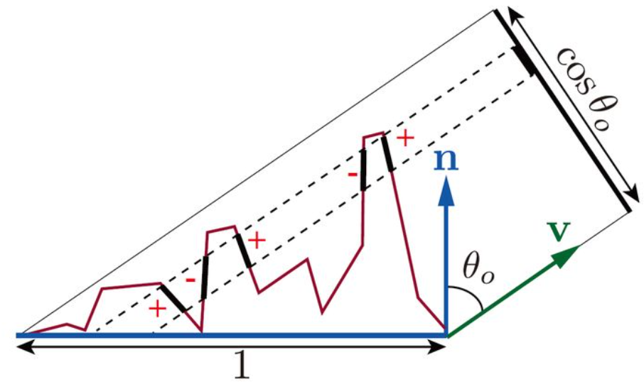
有，
$$
\int_{\Omega^+} D(\boldsymbol{h}) \space d\boldsymbol{h} \geq 1 \tag{2} \label{NDF Int}
$$

$$
\int_{\Omega^+} D(\boldsymbol{h}) \cos\theta_h \space d\boldsymbol{h} = 1 \tag{3} \label{NDF Projected Area}
$$

因此蒙特卡洛积分重要性采样的概率密度要依据 $D(\boldsymbol{h}) \cos\theta_h$ 设定，但蒙特卡洛积分是对入射光方向 $\boldsymbol{l}$，而 $D(\boldsymbol{h}) \cos\theta_h$ 是微表面法线的概率密度。但计算 BRDF 只需要关注能够反射到观察方向的入射光方向即可，而反射过程与微表面法线具有反射定律的关系，可以根据此关系推导出入射光方向 $\boldsymbol{l}$ 的概率密度。下面介绍几种微表面分布函数，

2.3.1 Blinn Phong NDF

$$
D_p(\boldsymbol{h})=\frac{\alpha_p+2}{2\pi}(\cos\theta_h)^{\alpha_p}
$$

其中 $\alpha_p$ 表示表面的光滑程度，当为 $\infty$ 时，表示绝对光滑表面。该参数带来的视觉变换非常不线性，不便调控。 UE4 中使用映射 $\alpha_p=2\alpha^{-2}-2$ ，$\alpha$ 为 roughness。

2.3.2 Beckmann NDF

$$
D_b(\boldsymbol{h})=\frac{1}{\pi\alpha^2(\cos\theta_h)^4}\cdot exp(\frac{\cos^2\theta_h-1}{\alpha^2\cos^2\theta_h})
$$

2.3.3 GGX(Trowbridge-Reitz) NDF

$$
D_{GGX}(\boldsymbol{h})=\frac{\alpha^2}{\pi((\cos\theta_h)^2(\alpha^2-1)+1)^2}
$$

3 根据 NDF 得到蒙特卡洛积分的重要性采样概率密度

求 $\eqref{BRDF MC}$ 中的积分，需要一个关于入射方向的概率密度函数 $p(\boldsymbol{l})$。$p(\boldsymbol{l})$ 无法直接获取，需要通过微表面法线概率密度函数得到。 因此第一步是先求得微表面法线概率密度函数 $p(\boldsymbol{h})$。

3.1 NDF 到微表面法线 PDF、CDF

由 $\eqref{NDF Int}$ 可知，NDF 并不是真正的概率密度函数，因为其在定义域的积分 $\geq1$ ，而 $\eqref{NDF Projected Area}$ 中的 $D(\boldsymbol{h})\cos\theta_h$ 才是真正的概率密度。对微表面法线概率密度 $p(\boldsymbol{h})$ 进行球坐标参数化有：

对于 $z$ 坐标轴为宏平面法线 $\boldsymbol{n}$ 的 hemisphere，$\boldsymbol{h}$ 的球坐标为 $(\phi_h,\theta_h)$，其中 $\phi_h \in [0,2\pi],\theta_h \in [0,\pi/2]$，并且 $\phi_h,\theta_h$ 相互独立。NDF $D(\boldsymbol{h})$ 对应的概率密度函数 PDF 为
$$
p_{\boldsymbol{h}}(\phi_h,\theta_h)=D(\boldsymbol{h})\cos\theta_h=D(\phi_h,\theta_h)\cos\theta_h
$$
计算机中的采样只能通过伪随机数生成服从均匀分布 $ U [0,1]$ 的采样点，需要通过变换转到服从其他分布的采样点 [2]。对于本文过程如下：在 $[0,1]\times[0,1]$ 进行均匀采样得到 $(x,y)$，用以表示采样点 $\boldsymbol{h}k(\phi{h_k},\theta_{h_k})$ 的概率，即
$$
P_k(\boldsymbol{h}k)=P_k(\phi{h_k},\theta_{h_k})=(x,y)
$$
$\eqref{NDF Projected Area}$ 为概率密度在随机变量的值域上的积分，将该积分的积分的微分立体角 $d\boldsymbol{h}$ 转换为球坐标有 $sin\theta_h\space d\phi_h d\theta_h$

计算边缘概率密度 $p_{\boldsymbol{h}}(\phi_h),p_{\boldsymbol{h}}(\theta_h)$ 有，
$$
\begin{align}
p_{\boldsymbol{h}}(\phi_h) &= \int_0^{\pi/2} p_{\boldsymbol{h}}(\phi_h,\theta_h) \sin\theta_h \space d\theta_h \
p_{\boldsymbol{h}}(\theta_h) &= \int_0^{2\pi} p_{\boldsymbol{h}}(\phi_h,\theta_h) \sin\theta_h \space d\phi_h
\end{align}
$$
再对边缘概率密度 $p_{\boldsymbol{h}}(\phi_h),p_{\boldsymbol{h}}(\theta_h)$ 进行积分得到的边缘概率分布 $P_{\boldsymbol{h}}(\phi_h),P_{\boldsymbol{h}}(\theta_h)$ 联立方程，
$$
P_{\boldsymbol{h}}(\phi_{h_k}) = \int_0^{\phi_{h_k}} p_{\boldsymbol{h}}(\phi_h)\space d\phi_h = x \
P_{\boldsymbol{h}}(\theta_{h_k}) = \int_0^{\theta_{h_k}} p_{\boldsymbol{h}}(\theta_h)\space d\theta_h = y
$$
即可求得方程的解 $\phi_{h_k},\theta_{h_k}$，代入得到所求概率密度 $p_k(\boldsymbol{h}k) =p k(\phi{h_k},\theta{h_k})$。

3.2 常用的 NDF 到微表面法线 PDF、CDF 的推导

下面按照第一小节中的步骤推导几个常用的 NDF 对应的微表面法线的概率密度函数。

3.2.1 Blinn Phong NDF 到 PDF、CDF

Blinn Phong NDF 对应的概率密度为：
$$
p_{\boldsymbol{h}}(\theta_h,\phi_h)=D_p(\boldsymbol{h})\cos\theta_h=\frac{\alpha_p+2}{2\pi}(\cos\theta_h)^{\alpha_p+1}
$$

• 计算边缘概率密度
  $$
  \begin{align}
  p_{\boldsymbol{h}}(\phi_h) &= \int_0^{\pi/2} p_{\boldsymbol{h}}(\phi_h,\theta_h) \sin\theta_h \space d\theta_h=\int_0^{\pi/2} \frac{\alpha_p+2}{2\pi}(\cos\theta_h)^{\alpha_p+1}\sin\theta_h\space d\theta_h \
  &= -\int_0^{\pi/2}\frac{\alpha_p+2}{2\pi}(\cos\theta_h)^{\alpha_p+1} \space d(\cos\theta_h) = -\frac{1}{2\pi}(\cos\theta_h)^{\alpha_p+2}\bigg|_0^{\pi/2} \
  &= \frac{1}{2\pi}
  \end{align}
  $$

  $$
  \begin{align}
  p_{\boldsymbol{h}}(\theta_h) &= \int_0^{2\pi} p_{\boldsymbol{h}}(\phi_h,\theta_h) \sin\theta_h \space d\phi_h = \int_0^{2\pi} \frac{\alpha_p+2}{2\pi}(\cos\theta_h)^{\alpha_p+1} \sin\theta_h \space d\phi_h \
  &= (\alpha_p+2)(\cos\theta_h)^{\alpha_p+1} \sin\theta_h
  \end{align}
  $$

• 计算边缘概率分布
  $$
  \begin{align}
  P_{\boldsymbol{h}}(\phi_{h_k}) &= \int_0^{\phi_{h_k}} p_{\boldsymbol{h}}(\phi_h)\space d\phi_h = \int_0^{\phi_{h_k}} \frac{1}{2\pi} \space d\phi_h \
  &= \frac{\phi_{h_k}}{2\pi}
  \end{align}
  $$

  $$
  \begin{align}
  P_{\boldsymbol{h}}(\theta_{h_k}) &= \int_0^{\theta_{h_k}} p_{\boldsymbol{h}}(\theta_h)\space d\theta_h = \int_0^{\theta_{h_k}} (\alpha_p+2)(\cos\theta_h)^{\alpha_p+1} \sin\theta_h\space d\theta_h \
  &= -\int_0^{\theta_{h_k}} (\alpha_p+2)(\cos\theta_h)^{\alpha_p+1}\space d(\cos\theta_h) = -(\cos\theta_h)^{\alpha_p+2}\bigg|0^{\theta{h_k}} \
  &= 1-(\cos\theta_{h_k})^{\alpha_p+2}
  \end{align}
  $$

• 根据均匀分布的采样点 $(x,y)$ 得到 Blinn Phong NDF 的采样点
  $$
  \begin{cases}
  \frac{\phi_{h_k}}{2\pi} = x \
  1-(\cos\theta_{h_k})^{\alpha_p+2} = y
  \end{cases}
  $$

  $$
  \begin{cases}
  \phi_{h_k} = x\cdot 2\pi \
  \cos\theta_{h_k} = (1-y)^{\frac{1}{\alpha_p+2}}
  \end{cases} \tag{4}\label{Blinn Phong Sampled Microface Normal}
  $$

3.2.2 GGX NDF 到 PDF、CDF

GGX NDF 对应的概率密度为：
$$
p_{\boldsymbol{h}}(\theta_h,\phi_h)=D_{GGX}(\boldsymbol{h})\cos\theta_h=\frac{\alpha^2\cdot \cos\theta_h}{\pi((\cos\theta_h)^2(\alpha^2-1)+1)^2}
$$

• 计算边缘概率密度
  $$
  \begin{align}
  p_{\boldsymbol{h}}(\phi_h) &= \int_0^{\pi/2} p_{\boldsymbol{h}}(\phi_h,\theta_h) \sin\theta_h \space d\theta_h=\int_0^{\pi/2} \frac{\alpha^2\cdot \cos\theta_h}{\pi((\cos\theta_h)^2(\alpha^2-1)+1)^2} \sin\theta_h \space d\theta_h \
  &= -\int_0^{\pi/2} \frac{\alpha^2\cdot \cos\theta_h}{\pi((\cos\theta_h)^2(\alpha^2-1)+1)^2} \space d(\cos\theta_h) \
  &= -\frac{\alpha^2}{2\pi}\int_0^{\pi/2} ((\cos\theta_h)^2(\alpha^2-1)+1)^{-2} \space d(\cos\theta_h)^2 \
  &= \frac{\alpha^2}{2\pi(\alpha^2-1)}\cdot\frac{1}{(\cos\theta_h)^2(\alpha^2-1)+1}\bigg|_0^{\pi/2} \
  &= \frac{1}{2\pi}
  \end{align}
  $$

  $$
  \begin{align}
  p_{\boldsymbol{h}}(\theta_h) &= \int_0^{2\pi} p_{\boldsymbol{h}}(\phi_h,\theta_h) \sin\theta_h \space d\phi_h = \int_0^{2\pi} \frac{\alpha^2\cdot \cos\theta_h}{\pi((\cos\theta_h)^2(\alpha^2-1)+1)^2} \sin\theta_h \space d\phi_h \
  &= \frac{2\alpha^2\cdot\cos\theta_h\cdot\sin\theta_h}{((\cos\theta_h)^2(\alpha^2-1)+1)^2}
  \end{align}
  $$

• 计算边缘概率分布
  $$
  \begin{align}
  P_{\boldsymbol{h}}(\phi_{h_k}) &= \int_0^{\phi_{h_k}} p_{\boldsymbol{h}}(\phi_h)\space d\phi_h = \int_0^{\phi_{h_k}} \frac{1}{2\pi} \space d\phi_h \
  &= \frac{\phi_{h_k}}{2\pi}
  \end{align}
  $$

  $$
  \begin{align}
  P_{\boldsymbol{h}}(\theta_{h_k}) &= \int_0^{\theta_{h_k}} p_{\boldsymbol{h}}(\theta_h)\space d\theta_h = \int_0^{\theta_{h_k}} \frac{2\alpha^2\cdot\cos\theta_h\cdot\sin\theta_h}{((\cos\theta_h)^2(\alpha^2-1)+1)^2}\space d\theta_h \
  &= -\int_0^{\theta_{h_k}} \frac{2\alpha^2\cdot\cos\theta_h}{((\cos\theta_h)^2(\alpha^2-1)+1)^2}\space d(\cos\theta_h) \
  &= -\alpha^2\int_0^{\theta_{h_k}} \frac{1}{((\cos\theta_h)^2(\alpha^2-1)+1)^2}\space d(\cos\theta_h)^2 \
  &= \frac{\alpha^2}{(\alpha^2-1)}\cdot\frac{1}{(\cos\theta_h)^2(\alpha^2-1)+1}\bigg|0^{\theta{h_k}} \
  &= \frac{\alpha^2}{(\alpha^2-1)[(\cos\theta_{h_k})^2(\alpha^2-1)+1]}-\frac{1}{\alpha^2-1}
  \end{align}
  $$

• 根据均匀分布的采样点 $(x,y)$ 得到 GGX NDF 的采样点
  $$
  \begin{cases}
  \frac{\phi_{h_k}}{2\pi}=x \
  \frac{\alpha^2}{(\alpha^2-1)[(\cos\theta_{h_k})^2(\alpha^2-1)+1]}-\frac{1}{\alpha^2-1} = y
  \end{cases}
  $$

  $$
  \begin{cases}
  \phi_{h_k} = x\cdot 2\pi \
  \cos\theta_{h_k} = \sqrt{\frac{1-y}{(\alpha^2-1)y+1}}
  \end{cases} \tag{5}\label{GGX Sampled Microface Normal}
  $$

3.3 微表面法线概率密度函数到入射方向的概率密度（推导失败）

首先思考一个问题：假设已知概率密度 $p_1(u,v)$，并且存在变换 $s=s(u,v),t=t(u,v)$ ，求概率密度 $p_2(s,t)$ 。

由概率密度在随机变量的取值空间积分为 1，设 $(u,v)\in \Omega_1$，$(s,t)\in \Omega_2$有：
$$
\begin{align}
\int_{\Omega_1} p_1(u,v)\space dudv &= \int_{\Omega_2} p_2(s,t)\space dsdt \
&= \int_{\Omega_1}p_2\Big(s(u,v),t(u,v)\Big) \space ds(u,v)dt(u,v) \
&= \int_{\Omega_1}p_2\Big(s(u,v),t(u,v)\Big)\left|\frac{\part (s,t)}{\part (u,v)}\right| \space dudv
\end{align}
$$
因此有：
$$
p_1(u,v)=p_2\Big(s(u,v),t(u,v)\Big)\left|\frac{\part (s,t)}{\part (u,v)}\right| \tag{6} \label{Transform PDF}
$$
其中 $\Large \left|\frac{\part (s,t)}{\part (u,v)}\right|$ 为雅可比行列式的绝对值 [4]，
$$
\left|\frac{\part (s,t)}{\part (u,v)}\right|=\left|\frac{\part s}{\part u}\cdot \frac{\part t}{\part v}-\frac{\part s}{\part v}\cdot\frac{\part t}{\part u}\right|
$$
下面只需要找到入射方向 $\boldsymbol{l}$ 与微表面法线 $\boldsymbol{h}$ 的关系即可利用 $\eqref{Transform PDF}$ 来得到入射方向的概率密度。

$\boldsymbol{h}$ 的概率密度为 $p_\boldsymbol{h}(\boldsymbol{h})$，$\boldsymbol{l}$ 的概率密度为 $p_\boldsymbol{l}(\boldsymbol{l})$。对于 $z$ 坐标轴为宏平面法线 $\boldsymbol{n}$ 的 hemisphere区域 $\Omega^+$，有积分
$$
\int_{\Omega^+} p_\boldsymbol{h}(\boldsymbol{h}) \space d\boldsymbol{h}=\int_{\Omega^+} p_\boldsymbol{l}(\boldsymbol{l}) \space d\boldsymbol{l}
$$

使用球坐标表示有：
$$
\begin{cases}
\boldsymbol{l}=(\phi_l,\theta_l) \
\boldsymbol{h}=(\phi_h,\theta_h)
\end{cases}
$$

$$
\iint_{\Omega^+} p_\boldsymbol{h}(\phi_h,\theta_h) \sin\theta_h \space d\theta_hd\phi_h=\iint_{\Omega^+} p_\boldsymbol{l}(\phi_l,\theta_l) \sin\theta_l\space d\theta_ld\phi_l
$$

由于 $\boldsymbol{l}$ 与 $\boldsymbol{h}$ 位于同一平面内，因此 $\phi_l=\phi_h$；观察 [Fig 1](#Reflection Fig) 有，$\theta_l+\theta_h=\theta_v-\theta_h \$ 。因此，
$$
\begin{cases}
\phi_l=\phi_h \
\theta_l=\theta_v-2\theta_h
\end{cases}
$$
因此雅可比行列式有：
$$
\left|\frac{\part \phi_l}{\part \phi_h}\cdot \frac{\part \theta_l}{\part\theta_h}-\frac{\part \phi_l}{\part\theta_h }\cdot \frac{\part\theta_l}{\part \phi_h}\right|=\left|1\times(-2)-0\times 0\right|=2
$$

代入有：
$$
p_\boldsymbol{h}\sin\theta_h=2\cdot p_\boldsymbol{l}\sin\theta_l \
p_\boldsymbol{l} = \frac{p_\boldsymbol{h}}{2\sin\theta_l/\sin\theta_h}
$$
????

[3] 通过构造新的坐标系得到
$$
p_\boldsymbol{l}(\boldsymbol{l})=\frac{p_\boldsymbol{h}(\boldsymbol{h})}{4(\boldsymbol{l}\cdot \boldsymbol{h})}=\frac{p_\boldsymbol{h}(\boldsymbol{h})}{4(\boldsymbol{v}\cdot \boldsymbol{h})}
$$

4 最终的渲染方程积分

至此我们已经可以计算 $\eqref{BRDF MC}$ 的积分了，由上述可知
$$
p_{\boldsymbol{l}}(\boldsymbol{l})=\frac{p_\boldsymbol{h}(\boldsymbol{h})}{4(\boldsymbol{v}\cdot \boldsymbol{h})}=\frac{D(\boldsymbol{h})\cdot \cos\theta_h}{4(\boldsymbol{v}\cdot \boldsymbol{h})}
$$
$\eqref{BRDF MC}$ 中的 $p(\boldsymbol{l}k)$ 即为上式的 $p{\boldsymbol{l}}(\boldsymbol{l})$。假设第 $k$ 次均匀分布采样点为 $(x_k,y_k)\in[0,1]\times[0,1]$，经过 $\eqref{Blinn Phong Sampled Microface Normal}$ 与 $\eqref{GGX Sampled Microface Normal}$ 可以得到该采样点在 NDF 上对应的微表面法线 $\boldsymbol{h}_k$ ，有：
$$
p(\boldsymbol{l}_k)=\frac{D(\boldsymbol{h}k)\cdot \cos\theta{h_k}}{4(\boldsymbol{v}\cdot \boldsymbol{h}_k)}=\frac{D(\boldsymbol{h}_k)\cdot \boldsymbol{h}_k\cdot \boldsymbol{n}}{4(\boldsymbol{v}\cdot \boldsymbol{h}_k)}
$$
$\eqref{BRDF MC}$ 中第 $k$ 次采样结果代入上式有，
$$
\begin{align}
& \frac{L_i(\boldsymbol{l}_k)f(\boldsymbol{l}k,\boldsymbol{v})\cos\theta{l_k}}{p(\boldsymbol{l}_k)} \
&= \frac{L_i(\boldsymbol{l}_k)\cdot(\boldsymbol{l}_k\cdot\boldsymbol{n})}{p(\boldsymbol{l}_k)}\cdot \frac{F(\boldsymbol{l}_k,\boldsymbol{v})\cdot G(\boldsymbol{l}_k,\boldsymbol{v},\boldsymbol{h}_k)\cdot D(\boldsymbol{h}_k)}{4(\boldsymbol{n}\cdot \boldsymbol{l}_k)(\boldsymbol{n}\cdot \boldsymbol{v})} \
&= \frac{L_i(\boldsymbol{l}_k)\cdot(\boldsymbol{l}_k\cdot\boldsymbol{n})}{\frac{D(\boldsymbol{h}_k)\cdot (\boldsymbol{h}_k\cdot \boldsymbol{n})}{4\boldsymbol{v}\cdot \boldsymbol{h}_k}}\cdot \frac{F(\boldsymbol{l}_k,\boldsymbol{v})\cdot G(\boldsymbol{l}_k,\boldsymbol{v},\boldsymbol{h}_k)\cdot D(\boldsymbol{h}_k)}{4(\boldsymbol{n}\cdot \boldsymbol{l}_k)(\boldsymbol{n}\cdot \boldsymbol{v})} \
&= \frac{L_i(\boldsymbol{l}_k)\cdot(\boldsymbol{v}\cdot \boldsymbol{h}_k)}{(\boldsymbol{h}_k\cdot \boldsymbol{n})}\cdot \frac{F(\boldsymbol{l}_k,\boldsymbol{v})\cdot G(\boldsymbol{l}_k,\boldsymbol{v},\boldsymbol{h}_k)}{(\boldsymbol{n}\cdot \boldsymbol{v})} \
&= \frac{L_i(\boldsymbol{l}_k)\cdot F(\boldsymbol{l}_k,\boldsymbol{v})\cdot G(\boldsymbol{l}_k,\boldsymbol{v},\boldsymbol{h}_k)\cdot (\boldsymbol{v}\cdot \boldsymbol{h}_k)}{(\boldsymbol{h}_k\cdot \boldsymbol{n})\cdot (\boldsymbol{n}\cdot \boldsymbol{v})}
\end{align}
$$
由上式可知，最终 BRDF 中的 NDF 项被舍去。

Reference

[1] [Real-Time Physically Based Material Basics](./2. Real-Time Physically Based Material Basics)

[2] [Introduction of Sampling in Computer](../Sample Algorithm/2. Introduction of Sampling in Computer.md)

[3] https://www.graphics.cornell.edu/~bjw/wardnotes.pdf

[4] [Jacobian Matrix](../Math/Jacobian Matrix.md)

[5] https://www.pbr-book.org/3ed-2018/Monte_Carlo_Integration/Importance_Sampling#sec:importance-sampling